Decision Trees
Decision Trees
1. What Is a Decision Tree?
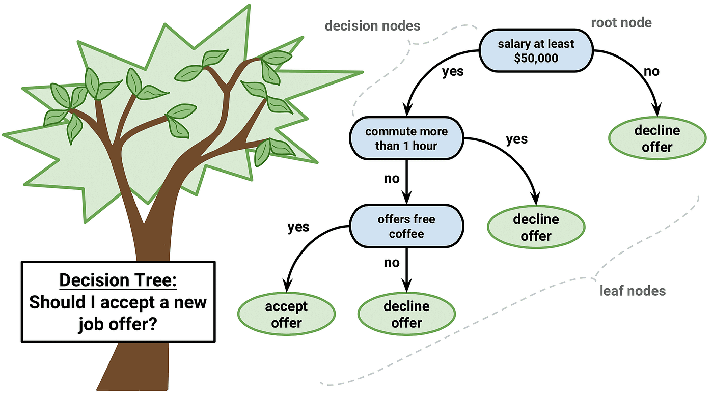
A Decision Tree is a supervised machine learning algorithm that models decisions as a hierarchical tree of binary (or multi-way) questions. Each internal node asks a question about a feature. Each branch is a possible answer. Each leaf node delivers a prediction — a class label (Classification) or a numeric value (regression).
It is one of the oldest, most studied, and most interpretable machine learning models. Its genealogy spans decades:
| Algorithm | Year | Key Innovation |
|---|---|---|
| ID3 | 1986 | Entropy / Information Gain (Quinlan) |
| C4.5 | 1993 | Gain Ratio, handles continuous features |
| CART | 1984 | Gini impurity, regression trees, pruning |
| C5.0 | 1997 | Faster, more memory-efficient than C4.5 |
CART (Classification and Regression Trees) is the algorithm behind sklearn's DecisionTreeClassifier and DecisionTreeRegressor, and forms the base of Random Forests and Gradient Boosted Trees.
2. The Core Geometric Intuition
Every split a decision tree makes draws a vertical or horizontal line through the feature space (axis-aligned split). The tree recursively partitions the space into rectangular regions, and each region gets a single prediction.
         x₂
          │
    ■ ■   │   ● ●
    ■ ■   │   ● ●
  ────────┼────────── x₁
    ● ●   │   ■ ■
    ● ●   │   ■ ■
          │
A decision boundary like this — where all splits are parallel to the axes — is called a rectilinear or axis-aligned boundary. This is fundamentally different from SVM (which draws angled hyperplanes) or Logistic Regression (which draws any linear boundary at any angle).
Consequence: Decision trees struggle with diagonal decision boundaries. A boundary like x₁ + x₂ = 1 requires many axis-aligned splits to approximate, while Logistic Regression does it in one step. But trees excel at capturing rectangular regions, step functions, and interaction effects between features.
3. Anatomy of a Decision Tree
                    ┌─────────────────┐
                    │   Root Node      │   ← Asks the most informative question
                    │  Age ≤ 35?       │
                    └────────┬────────┘
                   YES /     │     \ NO
                      /      │      \
           ┌──────────┐           ┌──────────┐
           │ Internal  │           │ Internal  │
           │Income≤50k?│           │ Credit≥7? │
           └─────┬─────┘           └─────┬─────┘
           /     │  \               /    │   \
         YES    NO               YES        NO
          │      │                │          │
      ┌───┴──┐ ┌─┴────┐       ┌───┴──┐  ┌───┴──┐
      │ Leaf │ │ Leaf  │       │ Leaf │  │ Leaf  │
      │ DENY │ │APPROVE│       │APPROVE│ │ DENY  │
      └──────┘ └──────┘       └──────┘  └──────┘
| Component | Description |
|---|---|
| Root Node | The first split; the single most informative feature |
| Internal Node | A split on a feature; has children |
| Branch | The edge connecting a node to its child (outcome of a test) |
| Leaf Node | Terminal node; delivers the final prediction |
| Depth | Length of the longest path from root to leaf |
| Split Point | The threshold used at an internal node (e.g., Age ≤ 35) |
| Subtree | A node and all of its descendants |
Depth = 1 is called a decision stump — a single split, one question. Despite being shallow, stumps are the base learners in many boosting algorithms (AdaBoost).
4. Mathematical Foundation — Splitting Criteria
The central question at every node: which feature, and which threshold, produces the best split?
"Best" is measured by how much a split reduces impurity — how much it moves the resulting child nodes from mixed classes toward pure classes (all one class).
4.1 Information Gain & Entropy (ID3)
Entropy measures the disorder or uncertainty in a set of labels:
H(S) = − Σₖ pₖ · log₂(pₖ)
Where pₖ is the fraction of samples belonging to class k.
Properties of entropy:
| Distribution | Entropy H(S) |
|---|---|
| All same class (pure) | H = 0 bits |
| 50/50 split (2 classes) | H = 1 bit |
| Uniform over K classes | H = log₂(K) bits |
Information Gain measures how much entropy a split removes:
IG(S, A) = H(S) − Σᵥ (|Sᵥ| / |S|) · H(Sᵥ)
Where:
S= current dataset at this nodeA= the feature being evaluatedSᵥ= the subset of S where feature A = value v|Sᵥ| / |S|= weight by fraction of samples in each child
We choose the split that maximizes Information Gain.
Worked Example:
Parent node: 10 samples → [6 positive, 4 negative]
H(parent) = −(6/10)log₂(6/10) − (4/10)log₂(4/10)
           = −0.6·(−0.737) − 0.4·(−1.322)
           = 0.442 + 0.529 = 0.971 bits

After split on feature A:
  Left child:  5 samples → [5 pos, 0 neg]  → H = 0
  Right child: 5 samples → [1 pos, 4 neg]  → H = 0.722

IG = 0.971 − (5/10)·0 − (5/10)·0.722
   = 0.971 − 0.361 = 0.610 bits
Higher IG → better split.
Weakness of Entropy / ID3: Biased toward features with many distinct values. A feature like "Customer ID" (all unique) would have maximum information gain (perfectly split data) but is useless for generalization. This is corrected by Gain Ratio.
4.2 Gini Impurity (CART)
Gini Impurity measures the probability that a randomly chosen element would be incorrectly classified if labeled randomly according to the class distribution:
Gini(S) = 1 − Σₖ pₖ²
Properties:
| Distribution | Gini |
|---|---|
| Pure node (one class) | Gini = 0 |
| 50/50 two classes | Gini = 0.5 |
| Uniform K classes | Gini = 1−1/K |
Gini Split Quality:
Gini_split = Σᵥ (|Sᵥ| / |S|) · Gini(Sᵥ)
We choose the split that minimizes Gini_split (equivalently, maximizes Gini reduction).
Comparison to Entropy:
- Gini is computationally cheaper (no logarithm)
- Gini tends to isolate the largest class in its own leaf
- Entropy tends to produce more balanced trees
- In practice, results are almost always identical — the choice rarely matters
Intuition: Gini = "probability of misclassifying a random point using the node's class distribution." A pure node never misclassifies → Gini = 0.
4.3 Gain Ratio (C4.5)
To correct entropy's bias toward high-cardinality features, C4.5 introduces the Split Information penalty:
SplitInfo(S, A) = − Σᵥ (|Sᵥ|/|S|) · log₂(|Sᵥ|/|S|)
Gain Ratio:
GainRatio(S, A) = IG(S, A) / SplitInfo(S, A)
A feature with many distinct values has high SplitInfo → Gain Ratio is penalized. This prevents overfitting to high-cardinality identifiers like IDs or timestamps.
Weakness: Gain Ratio can become unstable when SplitInfo is very small (e.g., binary features with very unequal splits). C4.5 addresses this by only considering features whose raw Information Gain exceeds the mean.
4.4 Comparing the Criteria
| Criterion | Formula Type | Task | Bias | Speed |
|---|---|---|---|---|
| Entropy (ID3) | Logarithmic | Classification | High-cardinality feat. | Moderate |
| Gini (CART) | Quadratic | Classification | Largest class | Fast |
| Gain Ratio (C4.5) | Ratio | Classification | More balanced | Moderate |
5. How It Works — The Splitting Algorithm
5.1 Greedy Search
Decision tree induction is a greedy algorithm — it makes the locally optimal split at each node without backtracking or considering the global tree structure.
At each node:
1. For every feature f in the dataset:
   2. For every possible split threshold t of feature f:
      3. Compute the impurity reduction of split (f, t)
3. Select (f*, t*) = argmax impurity reduction
4. Split data into left (x[f] ≤ t*) and right (x[f] > t*) subsets
5. Recurse on each child
This is not globally optimal. A split that looks mediocre now might enable two excellent splits downstream. But finding the globally optimal tree is NP-hard, so greedy induction is the universal practical approach.
5.2 Handling Continuous Features
For a continuous feature (e.g., Age = 23, 31, 45, 52, 67), candidate split thresholds are the midpoints between consecutive sorted unique values:
Sorted values: [23, 31, 45, 52, 67]
Candidate thresholds: [27, 38, 48.5, 59.5]
Only the midpoints between values where the label changes are informative — many implementations optimize by only evaluating those. With m training samples, there are at most m−1 candidate thresholds per feature, leading to O(m·p·log m) training complexity (p = number of features).
5.3 Handling Categorical Features
For a categorical feature with K categories:
Binary split (CART): Try all 2^(K−1) − 1 possible subsets of categories for the left child. For large K, this becomes exponential — in practice, one-hot encode or use frequency-based ordering tricks.
Multi-way split (C4.5/ID3): Create one branch per category value. This can lead to very fragmented nodes with few samples.
Ordinal categories: Treat as ordered → evaluate thresholds like continuous features.
5.4 Handling Missing Values
| Strategy | Description |
|---|---|
| Surrogate splits (CART) | Learn a backup split using another feature that mimics the primary split |
| Fractional assignment | Send the sample down all branches weighted by fraction of training data |
| Imputation beforehand | Fill in missing values with mean/mode before training |
| Ignore (sklearn default) | Samples with missing values are excluded from impurity computation |
C4.5's fractional approach is theoretically sound but adds complexity. CART's surrogate splits are elegant and production-proven.
6. How It Is Trained — Full Algorithm
function BuildTree(S, features, depth):

    # Stopping conditions
    if all samples in S have the same label:
        return Leaf(label)
    if features is empty OR depth == max_depth:
        return Leaf(majority_class(S))
    if |S| < min_samples_split:
        return Leaf(majority_class(S))

    # Find best split
    best_feature, best_threshold = None, None
    best_gain = −∞

    for each feature f in features:
        for each threshold t in candidate_thresholds(S, f):
            gain = impurity_reduction(S, f, t)
            if gain > best_gain:
                best_gain = gain
                best_feature, best_threshold = f, t

    # If no beneficial split found
    if best_gain == 0:
        return Leaf(majority_class(S))

    # Partition data
    S_left  = {x ∈ S : x[best_feature] ≤ best_threshold}
    S_right = {x ∈ S : x[best_feature] >  best_threshold}

    # Recurse
    left_child  = BuildTree(S_left,  features, depth + 1)
    right_child = BuildTree(S_right, features, depth + 1)

    return InternalNode(best_feature, best_threshold, left_child, right_child)
Time Complexity:
| Phase | Complexity |
|---|---|
| Training | O(m · p · log m · depth) |
| Prediction | O(depth) |
| Memory | O(m) (for the tree structure) |
Prediction is extremely fast — just traverse from root to leaf, O(log m) for balanced trees.
7. Stopping Criteria & Tree Depth
Without stopping criteria, a decision tree will grow until every leaf is pure — every sample correctly classified. This produces severe overfitting.
| Stopping Criterion | Parameter (sklearn) | Effect |
|---|---|---|
| Maximum depth | max_depth |
Hard cap on tree depth |
| Minimum samples to split | min_samples_split |
Node must have ≥ N samples to be split |
| Minimum samples per leaf | min_samples_leaf |
Each resulting leaf must have ≥ N samples |
| Minimum impurity decrease | min_impurity_decrease |
Split only if gain ≥ threshold |
| Maximum leaf nodes | max_leaf_nodes |
Grows tree breadth-first up to N leaves |
Interaction between parameters:
Deep tree + low min_samples → Overfitting
Shallow tree + high min_samples → Underfitting

Sweet spot: tune max_depth (3–10) + min_samples_leaf (5–50) together via CV
Rule of thumb for max_depth:
depth=1: Stump (for boosting base learners)depth=3–5: Interpretable, good generalizationdepth=10–20: More expressive, risk of overfittingdepth=None: Full tree (always overfit without pruning)
8. Pruning
Pruning is the process of removing parts of the tree that do not improve generalization — essentially undoing some splits made during training.
8.1 Pre-Pruning (Early Stopping)
Stop splitting early using the stopping criteria from Section 7. Simple and efficient, but may stop too early and miss beneficial later splits.
8.2 Post-Pruning (Cost-Complexity Pruning)
CART's approach — also called Minimal Cost-Complexity Pruning or Weakest Link Pruning. Grow the full tree first, then prune.
Define a cost-complexity measure for a subtree T rooted at node t:
Rα(T) = R(T) + α · |T|
Where:
R(T)= training error of the subtree (misClassification rate or total impurity)|T|= number of leaf nodes in the subtreeα= complexity penalty (regularization)
For each internal node, compute the effective alpha — the value of α at which pruning this subtree becomes worthwhile:
αeff(t) = [R(t) − R(Tₜ)] / [|Tₜ| − 1]
Where R(t) is the error of replacing the subtree with a single leaf, and R(Tₜ) is the error of the subtree.
Pruning procedure:
1. Grow the full tree T₀
2. Find the node t with the smallest αeff → prune it → T₁
3. Repeat to get a sequence: T₀ ⊃ T₁ ⊃ T₂ ⊃ ... ⊃ root
4. Use cross-validation to select the optimal Tᵢ
In sklearn:
from sklearn.tree import DecisionTreeClassifier
path = clf.cost_complexity_pruning_path(X_train, y_train)
alphas = path.ccp_alphas

# Cross-validate to find best alpha
best_alpha = cross_validate_alphas(alphas, X_train, y_train)
clf_pruned = DecisionTreeClassifier(ccp_alpha=best_alpha)
Post-pruning almost always outperforms pre-pruning because it sees the full tree before deciding what to cut.
10. Feature Importance
One of decision trees' most valuable properties: they provide a natural measure of feature importance.
Impurity-based importance (sklearn default):
Importance(f) = Σₜ (nₜ/n) · [Impurity(t) − (nₜₗ/nₜ)·Impurity(tₗ) − (nₜᵣ/nₜ)·Impurity(tᵣ)]
Where the sum is over all nodes t where feature f is used for splitting. The importance is the total weighted impurity reduction contributed by that feature across the entire tree.
Normalized so that all importances sum to 1:
clf.feature_importances_ # Array of shape [n_features,]
Interpretation:
Feature Importances:
  Income:      0.42   ← Most informative
  Age:         0.28
  Credit Score:0.18
  Employment:  0.08
  Zip Code:    0.04
Caveats:
- Biased toward high-cardinality or continuous features (more split candidates)
- Can be misleading with correlated features — importance gets split between them
- Reflects training data structure, not necessarily causal importance
- For more reliable importance: use permutation importance or SHAP values
from sklearn.inspection import permutation_importance
result = permutation_importance(clf, X_test, y_test, n_repeats=30)
11. Assumptions of the Model
Unlike Logistic Regression or SVM, decision trees make remarkably few assumptions:
| Assumption / Property | Description |
|---|---|
| No linearity assumption | Can model any shape of decision boundary (given enough depth) |
| No distributional assumption | Features can be skewed, non-normal, multi-modal — trees don't care |
| No scale requirement | Splitting at thresholds is scale-invariant; no need to normalize |
| Monotonic transformations irrelevant | log(x) vs. x produces identical trees (same rank order of split candidates) |
| Handles mixed types natively | Continuous and categorical features in the same tree |
| Features used independently | Each split uses one feature at a time — no feature interactions in splits themselves |
| Implicit feature selection | Irrelevant features are simply never selected for splitting |
The key assumption is that the true decision boundary can be approximated well by axis-aligned splits — which is not always the case (see drawbacks).
12. Advantages
✅ Exceptional Interpretability
A shallow decision tree is the most human-readable model in ML. You can draw it on a whiteboard, walk a non-technical stakeholder through it, and get instant buy-in. Rules are explicit:
IF Age ≤ 35 AND Income > 50k THEN Approve
ELSE IF Credit Score ≥ 700 THEN Approve
ELSE Deny
✅ No Feature Preprocessing Required
Unlike SVM, Logistic Regression, or neural networks:
- No normalization or standardization needed
- No one-hot encoding of ordinal features required
- Handles a mix of continuous and categorical features natively
- Robust to outliers — a split threshold simply puts outliers in their own leaf
✅ Handles Non-Linear Relationships
With sufficient depth, a decision tree can approximate any function (piecewise constant). It naturally captures:
- Feature interactions (splitting on x₁ at one level, x₂ at another)
- Non-monotonic effects (values in a middle range behave differently)
- Threshold effects (a sharp change at one value)
✅ Implicit Feature Selection
Features that are not useful are never split on. The model builds in automatic feature selection — a feature with zero importance was never needed.
✅ Handles Missing Values
Via surrogate splits (CART) or fractional assignment (C4.5), trees can process incomplete data without imputation.
✅ Works on Both Classification and Regression
The same algorithm, just a different splitting criterion and leaf prediction.
✅ Fast Prediction
Prediction is O(depth) — typically O(log m) for balanced trees. Extremely fast at inference time.
✅ Probabilistic Output (Coarse)
Returns class fractions from leaves — a rough probability estimate without extra machinery.
✅ Foundation of Powerful Ensembles
Decision trees are the building blocks of some of the most powerful algorithms in ML: Random Forest, Gradient Boosted Trees (XGBoost, LightGBM, CatBoost), and AdaBoost.
13. Drawbacks & Limitations
❌ Overfitting — The Core Weakness
Without constraints, a decision tree will perfectly memorize the training data. This is its most fundamental limitation. Pruning, max_depth, and min_samples_leaf help, but a single tree almost always overfits relative to ensemble methods.
❌ High Variance
Small changes in the training data can produce completely different trees. A few different training samples might lead to a different root split — changing the entire structure downstream. This instability is the primary motivation for Random Forests (which average many trees to reduce variance).
❌ Axis-Aligned Boundaries Only
The rectilinear decision boundary is a fundamental constraint. A diagonal boundary like x₁ + x₂ = 1 requires infinitely many axis-aligned splits to approximate, while Logistic Regression handles it trivially. For such problems, trees are dramatically inefficient.
❌ Cannot Extrapolate
Regression trees predict the mean of training values in a leaf. For test data outside the range of training data, the tree predicts the extremal training value — it cannot extrapolate trends.
Training: Age 20–60 → Salary $30k–$120k
Test: Age 70 → Tree predicts max training salary ≠ true salary
❌ Biased Toward Dominant Classes
On imbalanced datasets, the majority class dominates leaves, and the tree may never build rules for the minority class. Requires class_weight='balanced' or resampling.
❌ Greedy — Not Globally Optimal
Because splits are chosen greedily, the tree may miss a globally better structure. A mediocre split at the root might enable two excellent splits below — but greedy search won't find it if the root split looked better locally.
❌ Poor Probability Calibration
Leaf class fractions are coarsely calibrated, especially for deep trees. The probability of a leaf with 9/10 training positives is not necessarily 0.9 on test data.
❌ Instability With Continuous Features
Small changes in the training set near a threshold can flip the chosen split, cascading different trees. This Sensitivity is the price of the greedy threshold search.
14. Decision Trees vs. Other Classifiers
| Classifier | Interpretable | Non-linear | No Scaling | Missing Data | Overfit Risk | Probabilistic |
|---|---|---|---|---|---|---|
| Decision Tree | ✅ Highest | ✅ | ✅ | ✅ | ❌ Highest | ⚠️ |
| Logistic Regression | ✅ High | ❌ | ❌ | ❌ | Low | ✅ |
| SVM (kernel) | ❌ | ✅ | ❌ | ❌ | Low | ❌ |
| Random Forest | ⚠️ Medium | ✅ | ✅ | ⚠️ | Low | ✅ |
| Gradient Boosting | ⚠️ Medium | ✅ | ✅ | ✅ (some) | Medium | ✅ |
| Naive Bayes | ✅ High | ❌ | ❌ | ✅ | Very Low | ✅ |
| Neural Network | ❌ | ✅ | ❌ | ❌ | Very High | ✅ |
| k-NN | ⚠️ | ✅ | ❌ | ❌ | Medium | ⚠️ |
15. Practical Tips & Gotchas
Start With a Shallow Tree for Interpretability
from sklearn.tree import DecisionTreeClassifier, export_text

clf = DecisionTreeClassifier(max_depth=4, min_samples_leaf=10)
clf.fit(X_train, y_train)
print(export_text(clf, feature_names=feature_names))
A max_depth=4 tree has at most 16 leaves — still readable by humans.
Visualize the Tree
from sklearn.tree import plot_tree
import matplotlib.pyplot as plt

plt.figure(figsize=(20, 10))
plot_tree(clf, feature_names=feature_names,
          class_names=['No', 'Yes'],
          filled=True, rounded=True)
plt.savefig('decision_tree.png', dpi=300)
Color intensity = class purity. Deeper blue/orange = purer node.
Tune max_depth and min_samples_leaf Together
from sklearn.model_selection import GridSearchCV

param_grid = {
    'max_depth':       [3, 4, 5, 6, 8, 10, None],
    'min_samples_leaf':[5, 10, 20, 50],
    'criterion':       ['gini', 'entropy']
}

grid = GridSearchCV(DecisionTreeClassifier(), param_grid,
                    cv=5, scoring='f1', n_jobs=-1)
grid.fit(X_train, y_train)
print(grid.best_params_)
Use Cost-Complexity Pruning
path = clf.cost_complexity_pruning_path(X_train, y_train)
alphas = path.ccp_alphas[:-1]   # Exclude the trivial root-only tree

scores = []
for alpha in alphas:
    clf_a = DecisionTreeClassifier(ccp_alpha=alpha)
    score = cross_val_score(clf_a, X_train, y_train, cv=5).mean()
    scores.append(score)

best_alpha = alphas[np.argmax(scores)]
final_clf = DecisionTreeClassifier(ccp_alpha=best_alpha).fit(X_train, y_train)
Handle Class Imbalance
clf = DecisionTreeClassifier(class_weight='balanced')
# or
clf = DecisionTreeClassifier(class_weight={0: 1, 1: 10})
Feature Importance vs. Permutation Importance
# Impurity-based (fast, but biased toward high-cardinality features)
importances = clf.feature_importances_

# Permutation-based (slower, but more reliable and unbiased)
from sklearn.inspection import permutation_importance
perm = permutation_importance(clf, X_test, y_test, n_repeats=20, random_state=42)
perm_importances = perm.importances_mean
Always prefer permutation importance for feature selection decisions.
Watch for Data Leakage
Decision trees are powerful enough to pick up on subtly leaky features. A feature with near-perfect importance is often a sign of data leakage — check if that feature would be available at prediction time.
Single Tree vs. Ensemble Decision Rule
If you need interpretability above all → Single tree (max_depth ≤ 5)
If you need best Accuracy on tabular data → [[XGBoost]] / [[LightGBM]]
If you need a fast, good default → Random Forest
If you're exploring features → Single tree for importance, then ensemble
16. When to Use It
Use a Decision Tree when:
- Interpretability is paramount — medical diagnosis, credit scoring, legal decisions, regulatory compliance
- You need to present rules to non-technical stakeholders
- No feature preprocessing is feasible (messy, mixed-type datasets)
- Your data has many categorical features with natural hierarchies
- You need a fast, explainable baseline before trying ensembles
- You're doing feature importance analysis to understand your data
- Missing values are common and imputation is undesirable
- Training data is small and you need something robust
Do NOT use a single Decision Tree when:
- Predictive [[Accuracy]] is the primary goal — use Random Forest or Gradient Boosting instead
- The decision boundary is diagonal or smoothly curved
- You need calibrated probabilities — leaf fractions are coarse estimates
- Your dataset is very large and you need ensemble-level performance
- You're working with images, audio, or text — deep learning dominates
Summary
┌────────────────────────────────────────────────────────────────┐
│                DECISION TREES AT A GLANCE                      │
├────────────────────────────────────────────────────────────────┤
│  CORE IDEA     Recursive greedy splitting by impurity          │
│  GEOMETRY      Axis-aligned rectangular partitions             │
│  TRAINING      Greedy: maximize impurity reduction at each node│
│  SPLITTING     Gini / Entropy / Variance Reduction             │
│  PREDICTION    Leaf: majority class (or mean for regression)   │
│  STRENGTH      Interpretable, no scaling, handles mixed types  │
│  WEAKNESS      Overfitting, high variance, no extrapolation    │
│  HYPERPARAMS   max_depth, min_samples_leaf, ccp_alpha          │
│  BEST FOR      Explainability, baselines, feature exploration  │
│  REAL POWER    As base learners in Random Forests & Boosting   │
└────────────────────────────────────────────────────────────────┘