Support Vector Machines (SVM)
Support Vector Machines — Deep Analysis
"Find the boundary that is most wrong about nothing."
Table of Contents
1. What Is a Support Vector Machine?
A Support Vector Machine (SVM) is a supervised machine learning algorithm primarily used for Classification, though it extends naturally to regression (SVR) and anomaly detection. It was developed by Vladimir Vapnik and colleagues at Bell Labs in the 1990s, rooted in the theoretical framework of Structural Risk Minimization and VC dimension from statistical learning theory.
The central idea: rather than just finding any boundary that separates classes, SVM finds the boundary that maximizes the margin — the gap between the two classes. This makes it the most geometrically principled classifier in classical machine learning.
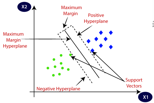
2. The Core Geometric Intuition
Imagine two classes of points plotted on a 2D plane — red circles and blue squares. Many lines could separate them. Which one should you choose?
  Blue  |      | Red
   ●    |      |    ■
  ●     |      |   ■
    ●   |  ←M→ |  ■
   ●    |      |    ■
SVM's answer: Choose the line that is furthest from both classes simultaneously — the one that maximizes the margin M. This is not just aesthetically pleasing; it has a deep justification:
-
A wider margin means the classifier generalizes better to unseen data
-
Points near the boundary are the most dangerous — a wide margin gives them more room
-
Maximizing margin is equivalent to minimizing generalization error (Vapnik's bound)
The points that sit exactly on the margin boundary and define it are called support vectors — the algorithm's namesake. Everything else in the dataset is irrelevant; remove any non-support-vector point and the solution doesn't change.
3. Mathematical Foundation
3.1 The Hyperplane
A hyperplane in n-dimensional space is defined by:
wᵀx + b = 0
Where:
wis the weight vector (normal to the hyperplane)bis the bias (shifts the hyperplane from the origin)xis a data point
For a 2D problem, this reduces to the familiar w₁x₁ + w₂x₂ + b = 0 — a line.
The signed distance of a point x from the hyperplane is:
distance = (wᵀx + b) / ||w||
This sign tells us which side of the hyperplane the point lies on — critical for Classification.
3.2 The Margin
We define two margin hyperplanes (gutters), one on each side of the decision boundary:
wᵀx + b = +1   (positive margin plane)
wᵀx + b = −1   (negative margin plane)
The geometric distance between these two planes is:
Margin M = 2 / ||w||
Maximizing M is equivalent to minimizing ||w|| (or ||w||² for mathematical convenience). This is the core of the optimization problem.
3.3 Support Vectors
Support vectors are the training points that satisfy:
wᵀxᵢ + b = +1   (closest positive-class points)
wᵀxᵢ + b = −1   (closest negative-class points)
These are the only points that matter for defining the decision boundary. In practice, typically only 5–30% of training data are support vectors.
This sparsity is a crucial property: SVM is a sparse model, defined entirely by a small subset of the training data.
3.4 The Optimization Problem (Hard Margin)
For perfectly linearly separable data, the optimization problem is:
Minimize:   (1/2) ||w||²

Subject to: yᵢ(wᵀxᵢ + b) ≥ 1   for all i = 1, ..., m
Where yᵢ ∈ {−1, +1} are the class labels (note: SVM uses ±1, not 0/1).
The constraint yᵢ(wᵀxᵢ + b) ≥ 1 means:
- For positive-class points (y=+1):
wᵀx + b ≥ +1✅ - For negative-class points (y=−1):
wᵀx + b ≤ −1✅
This is a convex quadratic program — it has a unique global minimum and can be solved efficiently.
4. Soft Margin SVM
Real-world data is almost never perfectly linearly separable. Hard margin SVM fails when:
-
Classes overlap (some misClassification is inevitable)
-
Data has outliers that would completely distort the boundary
-
A rigid boundary would have near-zero margin to achieve perfect separation
4.1 Slack Variables
We introduce slack variables ξᵢ ≥ 0 for each training point, allowing limited violations of the margin:
yᵢ(wᵀxᵢ + b) ≥ 1 − ξᵢ
Interpretation of ξᵢ:
| ξᵢ value | Meaning |
|---|---|
| ξᵢ = 0 | Point is correctly classified, outside or on margin |
| 0 < ξᵢ ≤ 1 | Point is inside the margin but correctly classified |
| ξᵢ > 1 | Point is misclassified (on the wrong side) |
4.2 The C Hyperparameter
The modified optimization problem becomes:
Minimize:   (1/2)||w||² + C · Σ ξᵢ

Subject to: yᵢ(wᵀxᵢ + b) ≥ 1 − ξᵢ,   ξᵢ ≥ 0
C controls the bias-variance tradeoff:
| C value | Behavior | Risk |
|---|---|---|
| C → ∞ | No violations tolerated → hard margin | Overfitting |
| C large | Few violations → narrow margin, complex boundary | Overfitting |
| C small | Many violations allowed → wide margin, simpler fit | Underfitting |
| C → 0 | Ignores all constraints → trivial solution | Underfitting |
Intuition: C asks "How much do I care about misclassifying training points?" High C = care a lot. Low C = prioritize a wide margin even if it costs some misClassifications.
Note: In sklearn, the hinge loss formulation uses C inversely to regularization — C = 1/λ.
5. The Kernel Trick
This is where SVM goes from a clever linear classifier to one of the most powerful non-linear classifiers in classical ML.
5.1 Why Kernels?
When data is not linearly separable in its original space, the intuition is:
Map the data into a higher-dimensional space where it is linearly separable.
Original 2D space (not separable) → Map to 3D → Now separable with a plane
A classic example: XOR data. Points at (0,0), (1,1) are Class A; (1,0), (0,1) are Class B. No line separates them in 2D. But add the feature x₃ = x₁·x₂ → the classes become linearly separable in 3D.
The problem: Mapping to very high (or infinite) dimensional spaces and computing dot products there is computationally catastrophic.
5.2 How the Kernel Trick Works
The SVM optimization (in its dual form — see Section 6) only ever uses data points through dot products xᵢᵀxⱼ.
The kernel trick replaces this with a kernel function:
K(xᵢ, xⱼ) = φ(xᵢ)ᵀ · φ(xⱼ)
Where φ(x) is the (potentially infinite-dimensional) feature mapping.
The magic: we never compute φ(x) explicitly. We only compute K(xᵢ, xⱼ) in the original input space, which is fast and efficient — but mathematically equivalent to operating in the transformed space.
Computation in original space:  K(xᵢ, xⱼ)   ← cheap
Implicit representation:         φ(xᵢ)ᵀφ(xⱼ) ← infinitely expensive if computed directly
A function K is a valid kernel if and only if it satisfies Mercer's condition: the kernel matrix K (where Kᵢⱼ = K(xᵢ, xⱼ)) must be positive semi-definite. This guarantees the kernel corresponds to some dot product in some feature space.
5.3 Common Kernel Functions
Linear Kernel
K(xᵢ, xⱼ) = xᵢᵀxⱼ
No transformation. Equivalent to standard SVM. Use when data is already linearly separable.
Polynomial Kernel
K(xᵢ, xⱼ) = (γ · xᵢᵀxⱼ + r)^d
d= degree of polynomialr= constant term (coef0 in sklearn)- Captures polynomial interactions between features
d=2adds quadratic features;d=3adds cubic; etc.
Radial Basis Function (RBF) / Gaussian Kernel
K(xᵢ, xⱼ) = exp(−γ · ||xᵢ − xⱼ||²)
- The most widely used kernel
- Implicitly maps to infinite-dimensional space
- Measures similarity as a Gaussian decay of Euclidean distance
γcontrols the "reach" of each support vector
| γ value | Effect |
|---|---|
| γ large | Narrow Gaussian → complex, wiggly boundary |
| γ small | Wide Gaussian → smooth, simple boundary |
Intuition: Each support vector "broadcasts" its influence over a Gaussian-shaped region. High γ = narrow influence = the model memorizes local structure.
Sigmoid Kernel
K(xᵢ, xⱼ) = tanh(γ · xᵢᵀxⱼ + r)
Resembles a neural network with one hidden layer. Not always positive semi-definite — use with caution.
5.4 Choosing a Kernel
Start → Is data high-dimensional and sparse?   → YES → Linear kernel
         ↓ NO
         Do you have domain knowledge of feature interactions? → YES → Polynomial
         ↓ NO
         Default: RBF kernel (grid-search γ and C)
         ↓
         Only try Sigmoid if motivated by neural network analogy
Rule of thumb: Always try Linear first (it's fastest). If performance is insufficient, try RBF with cross-validated hyperparameters.
6. How SVM Is Trained — The Dual Problem
6.1 Lagrangian Duality
SVM's training is formulated as a constrained optimization problem. The standard approach uses Lagrange multipliers to convert it into an unconstrained form called the Lagrangian:
L(w, b, α) = (1/2)||w||² − Σᵢ αᵢ[yᵢ(wᵀxᵢ + b) − 1]
Where αᵢ ≥ 0 are Lagrange multipliers — one per training example.
Setting partial derivatives to zero yields:
w = Σᵢ αᵢ yᵢ xᵢ        (weight vector as linear combo of training points)
Σᵢ αᵢ yᵢ = 0            (bias constraint)
Substituting back gives the dual problem:
Maximize:   Σᵢ αᵢ − (1/2) Σᵢ Σⱼ αᵢ αⱼ yᵢ yⱼ (xᵢᵀxⱼ)

Subject to: αᵢ ≥ 0,   Σᵢ αᵢ yᵢ = 0
Key insight: the dual depends on data only through dot products xᵢᵀxⱼ — exactly where kernels plug in.
6.2 KKT Conditions
The Karush-Kuhn-Tucker (KKT) conditions are the necessary and sufficient conditions for optimality:
αᵢ = 0        →  Point is NOT a support vector (correctly classified, outside margin)
0 < αᵢ < C   →  Point IS a support vector (exactly on the margin boundary)
αᵢ = C        →  Point violates the margin (inside margin or misclassified)
This gives SVM its sparsity: only points with αᵢ > 0 (support vectors) contribute to w. All other training points can be discarded post-training.
Prediction for a new point x:
f(x) = sign(Σᵢ αᵢ yᵢ K(xᵢ, x) + b)
This is computed using only the support vectors — elegant and efficient at inference time.
6.3 Solvers
| Solver | Algorithm | Best For |
|---|---|---|
| SMO | Sequential Minimal Optimization | General purpose (used in libSVM) |
| liblinear | Coordinate descent | Large-scale linear SVM |
| SDCA | Stochastic Dual Coordinate Ascent | Large datasets, online learning |
| Cutting-plane | Structural SVM | Structured output problems |
SMO (Platt, 1998) is the workhorse. It decomposes the QP into the smallest possible subproblems (pairs of αᵢ), each with a closed-form solution, iterating until convergence.
Time complexity: O(m²) to O(m³) for kernel SVM — this is the main scalability bottleneck.
7. SVM for Multiclass Classification
SVM is inherently a binary classifier. Two strategies extend it to K classes:
One-vs-One (OvO)
Train K(K−1)/2 binary classifiers — one for each pair of classes. Predict by majority vote.
For K=4: train classifiers for (1v2), (1v3), (1v4), (2v3), (2v4), (3v4)
→ 6 classifiers, each votes → take the majority
Advantage: Each classifier is trained on a small, balanced subset of data.
Disadvantage: Number of classifiers grows quadratically with K.
One-vs-Rest (OvR)
Train K binary classifiers: each class vs. all others. Pick the class with the highest decision score.
Advantage: Fewer classifiers (K vs K²/2).
Disadvantage: Training sets become imbalanced (1 class vs. K-1 classes).
sklearn default: OvO for SVC, OvR for LinearSVC.
8. Assumptions of the Model
| Assumption | Description |
|---|---|
| Separability (with margin) | Classes should be separable, at least with soft margin tolerance |
| Feature relevance | SVM assumes all features contribute — irrelevant features degrade the margin |
| No native probability calibration | Raw SVM scores are not probabilities; Platt scaling must be applied separately |
| Scale Sensitivity | Features must be on the same scale; SVM is not scale-invariant |
| Feature independence not required | Unlike Naive Bayes, SVM handles correlated features naturally |
| Appropriate kernel choice | The kernel must match the true structure of the data |
9. Evaluation Metrics
Since SVM is a classifier, standard Classificationon metrics]] apply. Note one critical difference from Logistic Regression:
SVM Has No Native Probabilities
Raw SVM produces a decision score f(x) = wᵀx + b, not a probability. To get probabilities:
# Platt scaling — fits a sigmoid to the SVM scores
model = SVC(probability=True)  # Adds cross-validation overhead
Platt scaling trains a Logistic Regression on top of SVM's decision scores. It works but adds computational cost and can be poorly calibrated.
Decision Function vs. Threshold
Predict +1  if  f(x) > 0
Predict −1  if  f(x) < 0
You can shift the threshold by adjusting b (the bias). This is useful in imbalanced settings.
Standard Metrics
Accuracy    = (TP + TN) / Total
[[Precision]]   = TP / (TP + FP)
Recall      = TP / (TP + FN)
[[F1-Score]]    = 2 · [[Precision]] · Recall / ([[Precision]] + Recall)
Hinge Loss
The native loss function of SVM, useful for monitoring training:
L_hinge = max(0, 1 − yᵢ · f(xᵢ))
- If
yᵢ · f(xᵢ) ≥ 1: point is correctly classified with margin → zero loss - If
yᵢ · f(xᵢ) < 1: point violates margin → positive loss
This is a convex upper bound on 0/1 loss. It is differentiable everywhere except at the "hinge" point.
10. Advantages
✅ Effective in High-Dimensional Spaces
SVM works extremely well when the number of features exceeds the number of samples (p >> n). Text Classification (tf-idf feature spaces) is a canonical example where SVM has historically dominated.
✅ Memory Efficient (Sparse Model)
The model is defined only by the support vectors — often a small fraction of training data. At prediction time, only support vectors participate in computation.
✅ Versatile via Kernels
By swapping kernels, SVM can model radically different decision boundaries — from linear to polynomial curves to Gaussian blobs — using the same underlying framework.
✅ Global Optimum Guaranteed
The objective is strictly convex (quadratic program). There are no local minima — gradient-based solvers always find the unique global solution.
✅ Strong Theoretical Guarantees
SVM minimizes the VC-dimension bound on generalization error. The margin is a direct measure of the model's generalization capacity — wider margin = lower VC dimension = better expected test performance.
✅ Robust to Overfitting in High Dimensions
Unlike many other models, SVM's complexity is controlled by the number of support vectors (not the number of features). It can generalize well even with many features.
✅ Works Well with Clear Margin Separation
When a clear gap exists between classes, SVM finds the optimal boundary with remarkable reliability.
✅ Kernel Flexibility
The kernel abstraction lets SVM operate on non-vectorial data — strings, graphs, sets — as long as a valid kernel can be defined.
11. Drawbacks & Limitations
❌ Scalability — The Achilles Heel
Training complexity is O(m²) to O(m³) in the number of training samples. For m = 100,000 points, this is computationally prohibitive with standard kernel SVM. Linear SVM (liblinear) scales to millions, but kernel SVM struggles beyond tens of thousands.
❌ No Native Probabilistic Output
SVM does not naturally output calibrated probabilities. Platt scaling helps but adds overhead and can be unreliable, especially with small datasets.
❌ Kernel and Hyperparameter Sensitivity
Choosing the right kernel and tuning C, γ, d, etc. requires expensive cross-validation. A poor kernel choice can result in very poor performance.
❌ Difficult to Interpret
Unlike Logistic Regression where coefficients have clear meaning, SVM coefficients in the dual space are not directly interpretable. With non-linear kernels, the model is essentially a black box.
❌ Sensitive to Feature Scaling
SVM with RBF kernel computes Euclidean distances. Features with large ranges dominate. Always scale before training.
❌ Sensitive to Noisy Data
SVM tries to maximize margin, which makes it sensitive to mislabeled points or overlapping distributions. Every noisy point that becomes a support vector directly distorts the boundary.
❌ Class Imbalance Handling is Manual
SVM does not naturally handle imbalanced classes. You must use class_weight='balanced' or resampling techniques.
❌ No Online Learning (for Kernel SVM)
Standard SVM requires the entire training set to be in memory. Incremental/online updates are non-trivial (though online SVM variants exist).
12. SVM vs. Other Classifiers
| Classifier | Non-linear | Probabilistic | Interpretable | Large Data | Scalable |
|---|---|---|---|---|---|
| SVM (kernel) | ✅ | ❌ | ❌ | ❌ | ❌ |
| SVM (linear) | ❌ | ❌ | ⚠️ | ⚠️ | ✅ |
| Logistic Regression | ❌ | ✅ | ✅ | ✅ | ✅ |
| Random Forest | ✅ | ✅ | ❌ | ✅ | ✅ |
| Neural Network | ✅ | ✅ | ❌ | ✅ | ✅ |
| k-NN | ✅ | ⚠️ | ⚠️ | ❌ | ❌ |
| Naive Bayes | ❌ | ✅ | ✅ | ✅ | ✅ |
| Decision Tree | ✅ | ⚠️ | ✅ | ✅ | ✅ |
13. Practical Tips & Gotchas
Always Scale Your Features
from sklearn.preprocessing import StandardScaler
scaler = StandardScaler()
X_train = scaler.fit_transform(X_train)
X_test = scaler.transform(X_test)
With RBF kernel, unscaled features make the kernel meaningless. Feature with range [0, 1000] will dominate feature with range [0, 1].
Hyperparameter Tuning — The Core Workflow
For RBF kernel, always tune both C and γ together:
from sklearn.model_selection import GridSearchCV
from sklearn.svm import SVC

param_grid = {
    'C':     [0.01, 0.1, 1, 10, 100],
    'gamma': ['scale', 'auto', 0.001, 0.01, 0.1],
    'kernel': ['rbf', 'poly', 'linear']
}

grid = GridSearchCV(SVC(), param_grid, cv=5, scoring='f1', n_jobs=-1)
grid.fit(X_train, y_train)
[[Start]] coarse, then fine-tune. A log-scale grid (powers of 10) is standard.
Getting Probabilities
model = SVC(probability=True)   # Enables Platt scaling
probs = model.predict_proba(X_test)
⚠️ This adds significant training time due to cross-validation for Platt scaling. Use decision_function() instead when probabilities are not needed.
Handling Class Imbalance
model = SVC(class_weight='balanced')
# or custom weights:
model = SVC(class_weight={0: 1, 1: 5})
When Your Dataset Is Large
For m > 10,000 samples, avoid kernel SVM. Use:
from sklearn.svm import LinearSVC          # Scales to millions
from sklearn.linear_model import SGDClassifier(loss='hinge')  # Online learning
Or use approximate kernels for a compromise:
from sklearn.kernel_approximation import RBFSampler
rbf_feature = RBFSampler(gamma=0.1, n_components=300)
X_approx = rbf_feature.fit_transform(X_train)
# Then train LinearSVC on X_approx
This approximates the RBF kernel with explicit (random) features — O(m) training time.
Diagnosing With the Decision Function
scores = model.decision_function(X_test)
# Positive scores → Class +1, Negative → Class −1
# |score| indicates confidence — magnitude, not probability
Plot the distribution of scores for each class to understand the margin and overlap.
Number of Support Vectors as a Health Check
print(model.support_vectors_.shape)
print(model.n_support_)
- Very few SVs (< 5% of data): Model may be too simple (low C or RBF too broad)
- Many SVs (> 50% of data): Model may be overfitting or data has poor separability
14. When to Use It
Use SVM when:
- You have a small-to-medium dataset (up to ~50,000 samples)
- Dimensionality is high and samples are relatively few (text Classification, bioinformatics)
- The margin between classes is clear (even if not perfectly separable)
- You need non-linear Classification and have time for kernel tuning
- You want a theoretically principled model with strong generalization bounds
- Working with non-standard data types (graphs, strings) with a custom kernel
- [[Accuracy]] matters more than interpretability
Do NOT use SVM when:
- Your dataset has more than ~50,000 samples (unless using LinearSVC or SGD)
- You need calibrated probabilities directly from the model
- You need fast retraining on streaming or changing data
- Interpretability is required by stakeholders or regulations
- You have many irrelevant or noisy features without prior selection
- You're working with images, audio, or text at scale — use deep learning
Summary
┌───────────────────────────────────────────────────────────────┐
│                  SVM AT A GLANCE                              │
├───────────────────────────────────────────────────────────────┤
│  CORE IDEA      Max-margin hyperplane between classes         │
│  KEY MATH       Convex QP via Lagrangian duality              │
│  TRAINING       SMO solver on dual problem                    │
│  DECISION       sign(Σ αᵢ yᵢ K(xᵢ, x) + b)                  │
│  POWER MOVE     Kernel trick → non-linear without mapping φ   │
│  STRENGTH       High-dim, small data, global optimum          │
│  WEAKNESS       Slow on large data, no probabilities          │
│  HYPERPARAMS    C (margin tolerance) + kernel params          │
│  BEST FOR       Text, bioinformatics, clean [[Classification]]     │
└───────────────────────────────────────────────────────────────┘